Data Engineering Zoomcamp — Week 3 (Data Warehouse)

Week 3 was about data warehousing, working on the data that was ingested in the week 2. We will take the already ingested data and create an external table from it and optimize the performance of queries through partitioning and clustering. Then automate the whole process using airflow.

There are two systems types when dealing with data: Online Transaction Processing (OLTP) and Online Analytical Processing (OLAP). OLTP systems are used when dealing with transaction-oriented applications. Data is stored in traditional databases. Examples of such systems are:

ATM
Shopping cart
MoMo
ticket systems

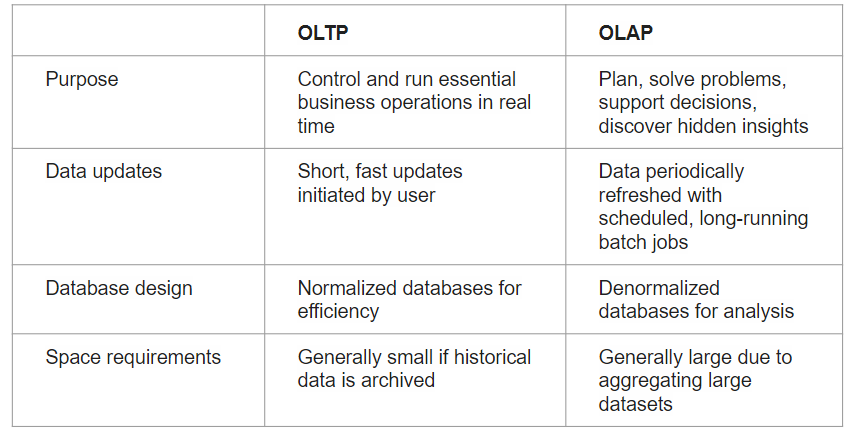
OLAP on the other hand is used for data analysis. Data is aggregated from multiple sources and used by the business team to make decisions. Example is data warehouse

OLAP VS OLTP

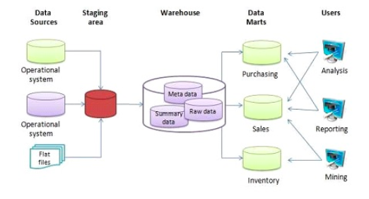
Data Warehouse

It differs from a data lake because it store transactional systems. Data structure and schema is defined in advance. The main goal is to become the single source of truth in an organization. It therefore combines data from multiple sources. It is used for reporting and data analysis. A use case can be a retail store with multiple branches acting as individual entities. This means that each branch has an instance of the application and database. The business team want to have a general look at the business, a data warehouse with consolidated data will work. This can apply to banks, factories and hotels.

BigQuery

An example of a data warehouse is BigQuery by Google. It is a serverless data warehouse meaning you do not manage servers or software. It has built in features such as machine learning, geospatial analysis and BI. It separates compute engine from storage, making it flexible for its customers.

There are two pricing models:

on-demand — $5 per 1TB and first 1TB per month is free
Flat Rate — Based on number of pre requested slots. Mostly for high volume customers. 100 slots → $2,000/month = 400 TB data processed on demand pricing

External Tables

This is a table that has its data residing in an external source. When one has files, they can create a table from it. They have the following limitations:

They are read-only
Does not guarantee data consistency
Query performance is not as high as native table
You cannot export data from external table
They do not support clustering

CREATE OR REPLACE EXTERNAL TABLE `de-first-340309.trips_data_all.external_yellow_tripdata` 
OPTIONS (
format = ‘parquet’,
uris = [‘gs://{bucket}/raw/yellow_tripdata/2019/*’,’gs://{bucket}/raw/yellow_tripdata/2020/*’]
);

Partitioning and Clustering data

“more data you scan, more you pay”. When using BigQuery, one should optimize cost by reducing read data in each query. To achieve this, one can use partitioning and/clustering.

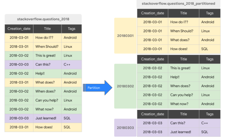
Partitioning a table is dividing it into segments that make make it easier to query data. This improves query performance and the amount of data that is scanned in a query. In BigQuery, one can partition a table by

Time-unit column — Timestamp, date, date time. It can be in days, hours minutes, months and years. Choosing which partitioning depends on the amount of data and the wide range.

Daily partition is the default. Best when data has a wide range of dates.

Hourly partitions are best when data has less that 6 months of timestamp. High volume of data over a short period of time

Monthly or yearly partitions is when data has small amount of data for each day.

Ingestion time
Integer range — start, end and an interval

Partitioning have limits of 4000 partitions.

When to use partitioning:

You want to know query costs before a query runs. Partition pruning is done before the query runs, so you can get the query cost after partitioning pruning through a dry run. Cluster pruning is done when the query runs, so the cost is known only after the query finishes.
You need partition-level management. For example, you want to set a partition expiration time, load data to a specific partition, or delete partitions.
You want to specify how the data is partitioned and what data is in each partition. For example, you want to define time granularity or define the ranges used to partition the table for integer range partitioning.

CREATE OR REPLACE TABLE de-first-340309.trips_data_all.yellow_tripdata_partitioned
PARTITION BY 
DATE(tpep_pickup_datetime) AS 
select * from de-first- 340309.trips_data_all.external_yellow_tripdata;

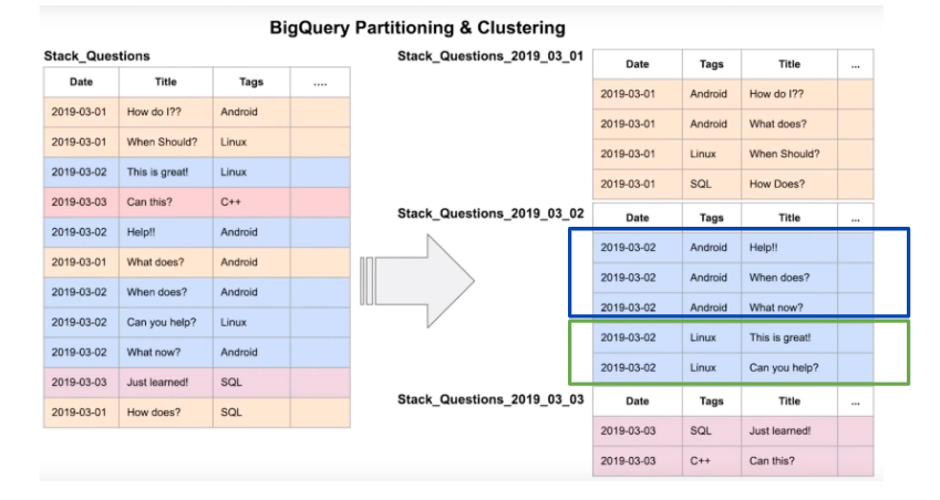
Clustering is done when filtering and aggregating is being done. One can use up to 4 columns when clustering. The order of the columns is important, hence the order of the specified column when clustering determines how the data is sorted.

Clustering can be done in the following non-repeated columns:

DATE
BOOL
GEOGRAPHY
INT64
NUMERIC
BIGNUMERIC
STRING
TIMESTAMP
DATETIME

create or replace table `de-first-340309.trips_data_all.yellow_tripdata_partitioned_clustered`
partition by DATE(tpep_pickup_datetime)
cluster by VendorID as
select * from de-first-340309.trips_data_all.external_yellow_tripdata;

When to use clustering:

You don’t need strict cost guarantees before running the query.
You need more granularity than partitioning alone allows. To get clustering benefits in addition to partitioning benefits, you can use the same column for both partitioning and clustering.
Your queries commonly use filters or aggregation against multiple particular columns.
The cardinality of the number of values in a column or group of columns is large.

Clustering over partitioning

Partitioning results in a small amount of data per partition (approximately less than 1 GB)
Partitioning results in a large number of partitions beyond the limits on partitioned tables
Partitioning results in your mutation operations modifying the majority of partitions in the table frequently (for example, every few minutes)

BigQuery best practices

To reduce cost, these are the best practices:

Avoid SELECT *
Price your queries before running them
Use clustered or partitioned tables
Use streaming inserts with caution
Materialize query results in stages

To increase query performances,

Filter on partitioned columns
Denormalizing data
Use nested or repeated columns
Use external data sources appropriately
Don’t use it, in case u want a high query performance
Reduce data before using a JOIN
Do not treat WITH clauses as prepared statements
Avoid oversharding tables

BigQuery and Airflow

Interactions with BigQuery can be automated using airflow. Airflow has operators by different operators. There is good documentation of the operators. An example is, creating an external table, one use BigQueryCreateExternalTableOperator from airflow.providers.google.cloud.operators.bigquery

From the above, this is just a tip of the iceberg. This is just a starting point. I will be looking deeper into each section later.